ONE HEALTH QUANTITATIVE METHODS
2.6
Matrix models of population dynamics
Populations are dynamic. They are influenced by different incidents, like for example birth and death. An illness can also change the number of individuals in a population. But how do we model a dynamic population? Let us examine this question for a One Health approach. If your browser runs into issues displaying the mathematical formulas, find attached a PDF of this article below.
Populations are dynamic
The phenomenon of infectious disease in populations is essentially a dynamic process at all levels. The susceptible host population is continuously changing through events such as birth, immigration, emigration and death. The parasite population is growing in the host, destroyed by the immune system or remains at low densities in reservoir hosts. The sum of all events may be expressed as a pool or a compartment, which is presented here with the example of a host population (see image one). The size of this compartment may be rising, declining, or oscillating. Even if the total size is stable, it may be highly dynamic. The above processes occur independently but simultaneously. They can be expressed in terms of the total population per time unit, ie as annual or instantaneous per capita birth rate $$b$$ or annual per capita mortality rate $$m$$. These rates themselves may be constant or dynamic. Populations may increase or decrease by constant rates of change.
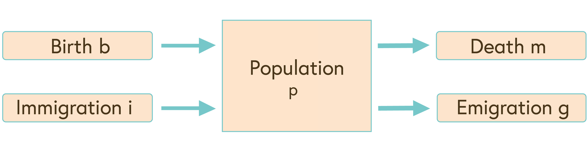
Image one: simple population flowchart
© Jakob Zinsstag
Population dynamics can be modeled
The dynamics of populations can be quantified as deterministic or stochastic processes. One could argue that models are always imperfect because of the complexity of nature. Nevertheless partial processes may very well be modeled with considerable precision. At best, models are aids to thought or frameworks for decision-making. It is essential that we properly identify the process we want to describe. For this we should establish its various elements as a flow chart (see image one). The basic rule is to ‘model what we can count’. For every countable item we draw a box. Arrows are used to connect compartments and indicate the direction of specific transitions such as birth, death, or infection. The resulting flow chart may be translated into mathematical equations. As a first step, an equation is written for every compartment.
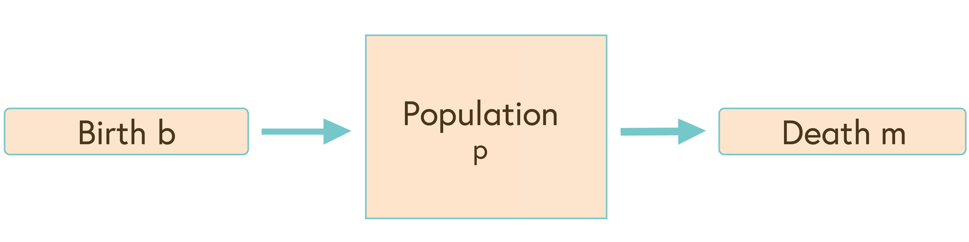
Image two: the isolated population $$P$$
© Jakob Zinsstag
Continuing with our first example, in image two we again describe the flow chart from image one, this time assuming the population is isolated and neither immigration nor emigration occurs. If we multiply the per capita rates with the population size, we obtain net birth rates $$bP$$ or net mortality rates $$mP$$. If the chosen time interval approaches zero, the dynamic of the total population can be expressed as a derivative $$\frac{dP}{dt}$$. The instantaneous rate of population change – which is proportional to the total population size (see equation one) – can be written as a differential equation (see equation two). The differential $$\frac{dP}{dt}$$ is the slope of the population function $$P(t)$$ over time:
Equation two describes the flow chart in image two but gives us no further information on the size of the population at a given time. Thus, we need to express the relationship in terms of the total population $$P$$ depending on birth and mortality. This can be achieved by an analytical solution of equation two, assuming that $$b$$ and $$m$$ are constant.
$$ ln P = (b - m)t + c \color{red}{→} P = e^{(b - m)t + c}$$ Equation three {.footnote-title}
Equation three is obtained by the integration of equation two and now expresses the population $$P$$ as a function of $$b$$ and $$m$$. $$C$$ is a constant which can be converted by writing the population size at time $$0$$. Thereby the time-dependent term is zero and the equation can be rewritten as
In image three the dynamics of a population $$ P_0 = 100$$ at year $$0$$ is plotted for a mortality rate of $$m = 0.05$$ per year and a birth rate $$b = 0.15$$ per year alone and for the total population $$P$$(birth-mort). The slope $$\frac{dP}{dt}$$ is added to the curve as a dashed line. This simple case has an analytical solution, but often more complex differential equations cannot be integrated using algebraic methods. In such cases computer programs are used to iteratively fit parameters to observed data and produce a numerical solution of the equation. Model parameters are often not constant. For example, mortality is age dependent. Younger individuals die more frequently than older. Parameters may also be density dependent, which means that the parameters are themselves again functions of the population.
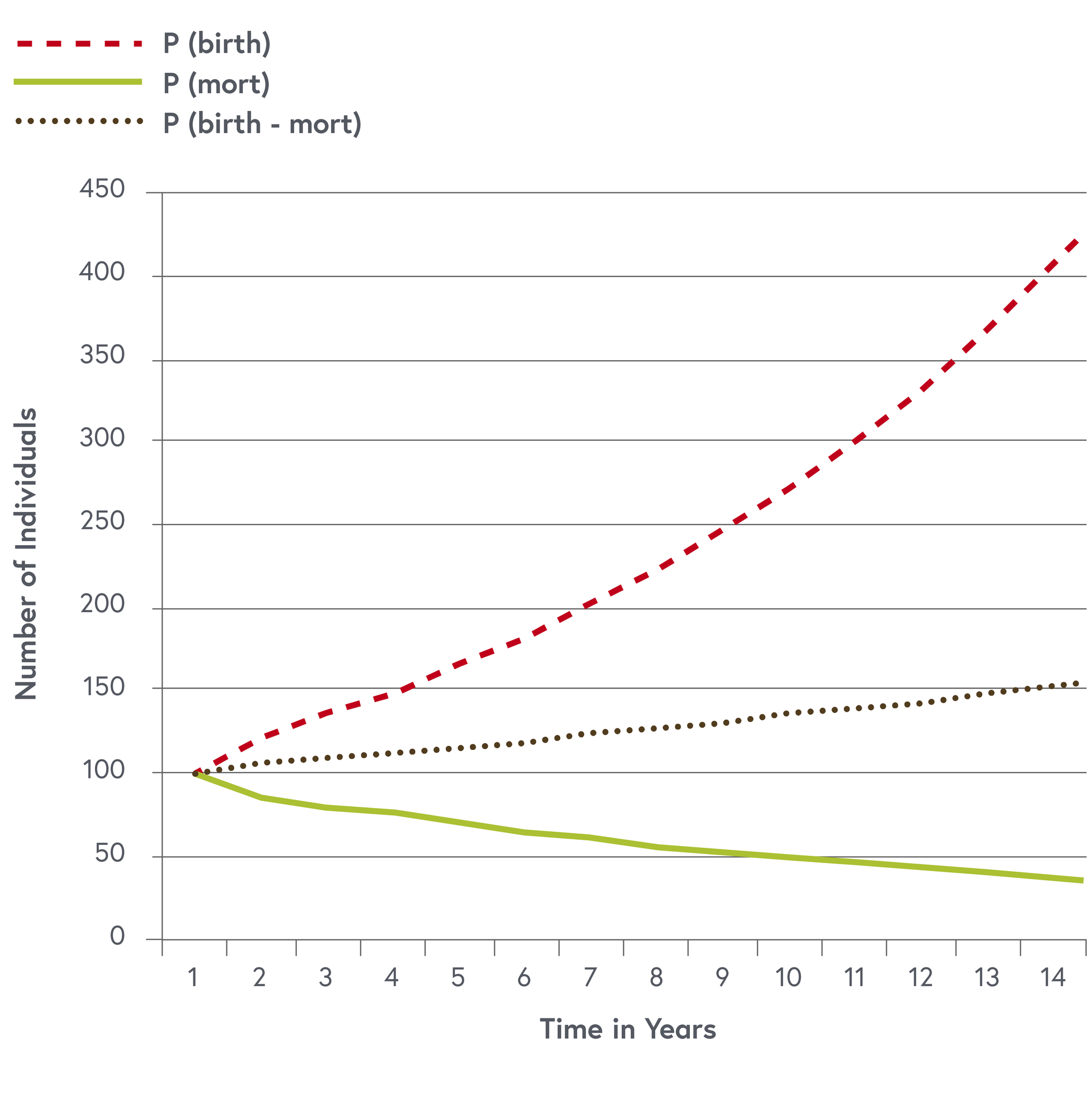
Image three: population dynamic with mortality and birth rates as independent processes
© Jakob Zinsstag
Modelling structured populations
Populations can be divided in genders and different age classes. An example is shown in image four, depicting an age and sex structured model of a cattle population in Mongolia. $$x$$ are female animals who give birth and $$y$$ are males.
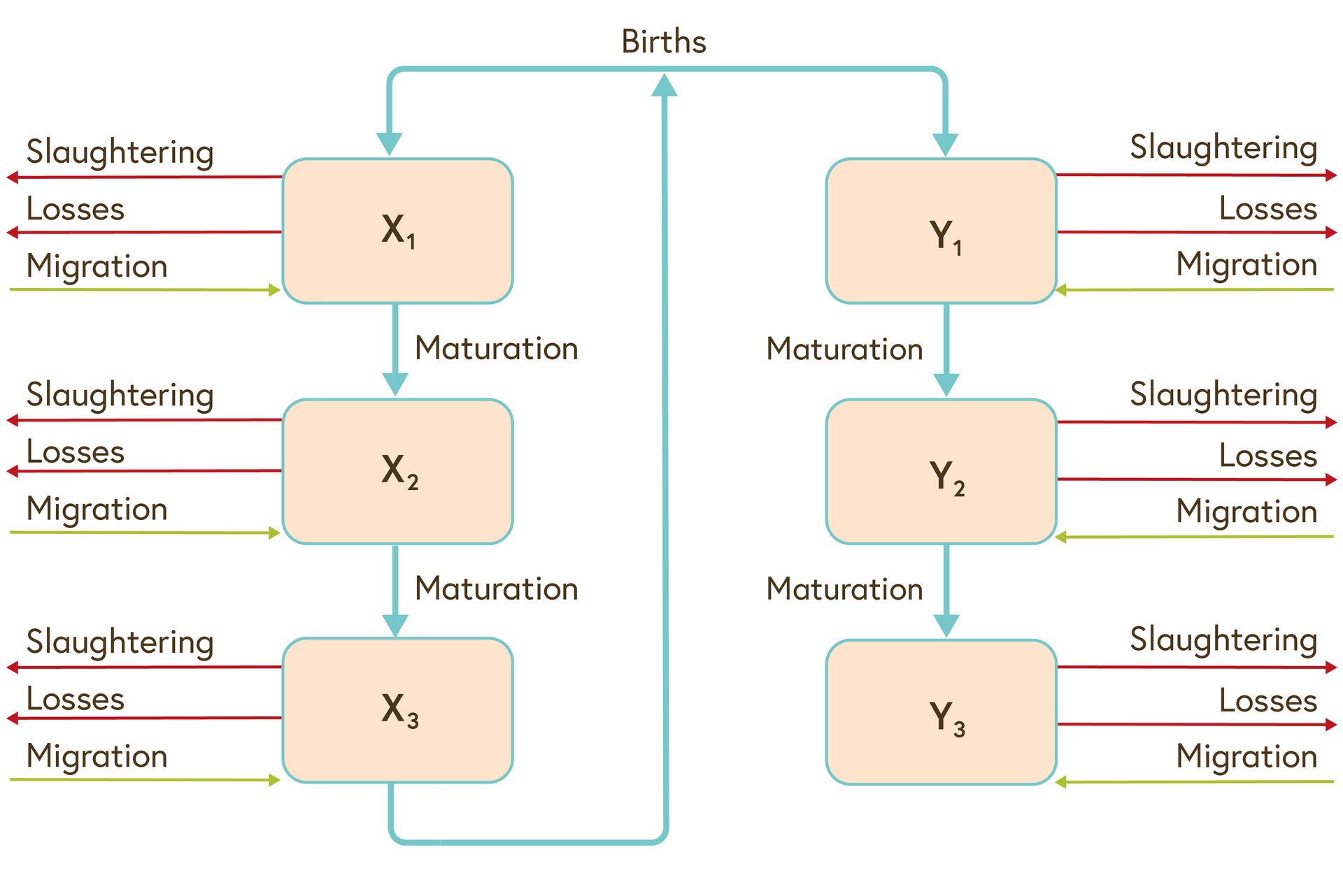
Image four: age and sex structured demographic model of a cow population
© adapted from Shabb et al. 2013, 280-288.
Such models can be simulated using differential or difference equations. They can also be modelled using matrix models. We introduce here the principle of the Leslie matrix which is widely applied in population dynamics. We follow the excellent introduction on the subject of population ecology by Vandermeer and Goldberg (Vandermeer and Goldberg 2008, 280pp).
The different classes of a population are no longer considered as a single value (scalar) but can be considered as a vector called population vector $$N$$. In this example, we consider three classes of female animals: young, subadult and adult (reproductive). This vector is multiplied by a projection matrix $$P$$.
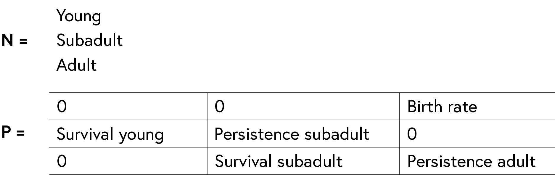
After a number of multiplications with itself, ie 20-30, the matrix reduces itself to diagonal values of $$\lambda$$, called the dominant Eigenvalue of the projection matrix $$P$$. Since $$P^n$$ is a diagonal matrix, we can replace it with $$\lambda^n$$.
The population structure becomes stable; the proportions between the vector elements are constant. The stabilised population vector becomes the Eigenvector. We can standardise the Eigenvector to a length of $$1$$, which is also called a normed Eigenvector.
References
J.H. Vandermeer and D.E. Goldberg (2003). Population Ecology: First principles. Princeton and Oxford, Princeton University Press.
Shabb et al. (2013). A Mathematical Model of the Dynamics of Mongolian Livestock Populations, in: Livestock Science 157, 280-288.
License
University of Basel
Downloads