Pattern recognition explains how the visual system extracts features from the retinal image, but it cannot resolve the fundamental ambiguity inherent in perception. The inverse problem of perception, however, cannot be resolved by bottom-up feature detection alone. To interpret ambiguous sensory data, the brain must draw on prior knowledge, and Bayesian inference gives us the mathematical language to describe how.

We have seen that pattern recognition provides an elegant means of constructing representations from sensory input. Yet its bottom-up architecture cannot solve the inverse problem of perception: many different physical scenes can produce the same retinal image. To interpret the world correctly, the brain must therefore incorporate prior knowledge about how the world typically behaves. Bayes’ theorem provides the mathematical framework for combining prior knowledge about the world with sensory evidence probabilistically:

Bayes’ theorem provides the mathematical framework for combining prior knowledge about the world with sensory data probabilistically:

The prior (expectation) encodes expectations about possible world states. For example, that light sources are usually white or yellowish, that objects are solid, or that faces are convex.

The likelihood (sensory data) captures how probable a given sensory input is, given a particular world state.

Combining prior and likelihood yields the posterior (the percept): our updated belief about the state of the world after taking the sensory evidence into account.

To illustrate the key intuition, take a look at the image below. In Bayesian inference, beliefs about the world are represented as probability distributions: rather than committing to a single answer, the brain maintains a spread of possibilities, each with some associated probability. The curves below show exactly this. The prior (purple) represents expectations about likely world states. The likelihood (teal) reflects the evidence from the sensory signal. The posterior (amber) is the outcome: a narrower distribution that sits between the two, weighted toward the more precise source. What we actually perceive here is the posterior. The posterior is weighted by precision (the inverse of variance), reflected in how narrow the curve is. In our example, the precise prior dominates the broader likelihood, pulling the posterior toward the expectation.

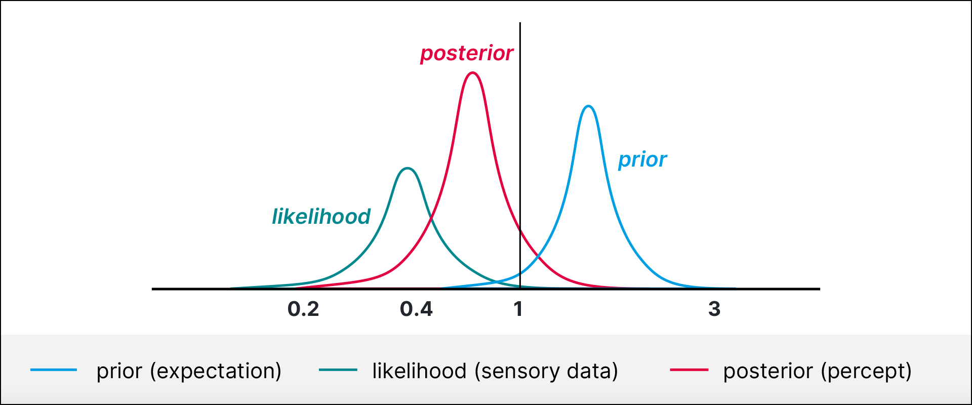
Bayes theorem

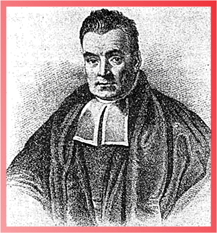
Thomas Bayes, 1701–1761

The core idea, as first articulated by Hermann von Helmholtz in the 1860s, is that the brain maintains an internal model of the world and works backwards from observations to infer their causes. Helmholtz called this process unconscious inference: the brain arrives at a percept not by passively reading out sensory data, but by generating hypotheses and testing them against incoming evidence.

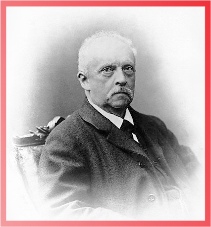
Hermann von Helmholtz, 1821–1894

This intuition sat largely dormant as a formal idea until researchers in speech perception picked it up in the 1960s. They noticed that recognizing spoken words seemed to work the same way: the mind generates candidate interpretations and checks them against the incoming sound. They called this analysis-by-synthesis. The label stuck, and the idea gradually spread to vision and perception more broadly.

What made it powerful was the realization, spelled out by Yuille and Kersten in 2006, that this is more than just a metaphor. Generating and evaluating candidate interpretations is precisely what Bayesian inference computes. The two frameworks turn out to describe the same process from different angles: one in computational terms, one in terms of what the brain might actually be doing.

Building on this idea, in 1999 neuroscientists Rajesh Rao and Dana Ballard proposed a specific neural architecture – predictive coding – in which the visual cortex embodies the logic of Bayesian inference.

The architecture works like this. Higher-level brain areas continuously send predictions downward: this is what I expect to see. Lower-level areas compare those predictions against the actual incoming signal. If the prediction was accurate, nothing much needs to travel back up. If it was wrong, the mismatch is sent upward. That mismatch is the prediction error.

This is a surprisingly economical design. The brain does not pass the full sensory signal up through every level of the hierarchy. It passes only the surprise, only what the model did not already anticipate. Everything expected is, in a sense, explained away before it gets any further.

Take a look at the figure below, which shows this architecture across three levels of the visual hierarchy.

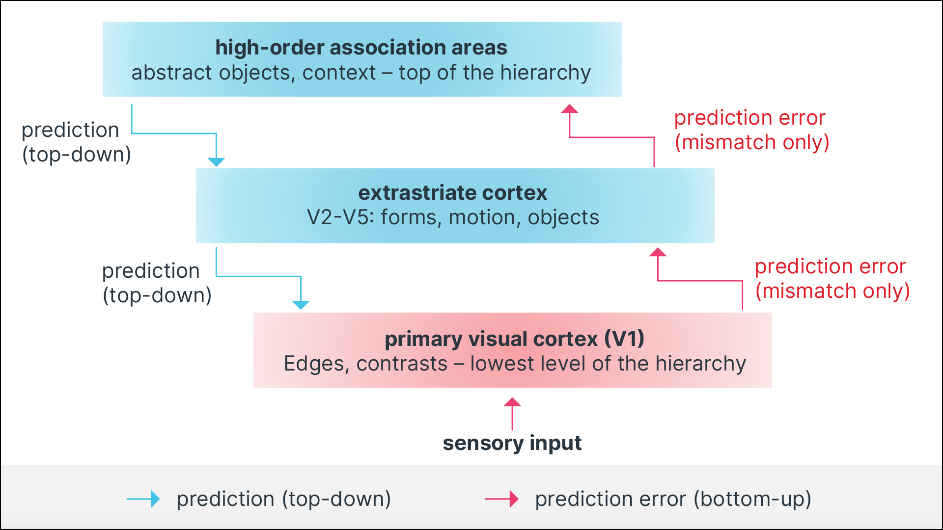
Predictive coding architecture (Rao & Ballard, 1999)
Higher areas predict; lower areas return only the mismatch – the prediction error.

Karl Friston extended this framework significantly in 2005. Where Rao and Ballard had focused on the visual cortex, Friston proposed that the same architecture could describe how the entire cerebral cortex works, across all sensory modalities and beyond.

In his formulation, every level of the cortical hierarchy carries a generative model: an internal representation capable of predicting the input it should receive from the level below. Perception, on this account, is not a single computation but an ongoing process. The hierarchy continually generates predictions, compares them against incoming signals, propagates errors upward, and revises its models. Prediction error is not a failure of the system. It is the engine that drives learning and updating.

A crucial refinement introduced by Friston is that not all prediction errors contribute equally to belief updating. The brain also estimates the reliability of each signal — its precision, a measure of how reliable or trustworthy a signal is.

A highly reliable signal (high precision, narrow distribution) should drive a large update to the internal model. An unreliable signal (low precision, broad distribution) should be discounted. This precision weighting acts as a gain control on incoming prediction errors.

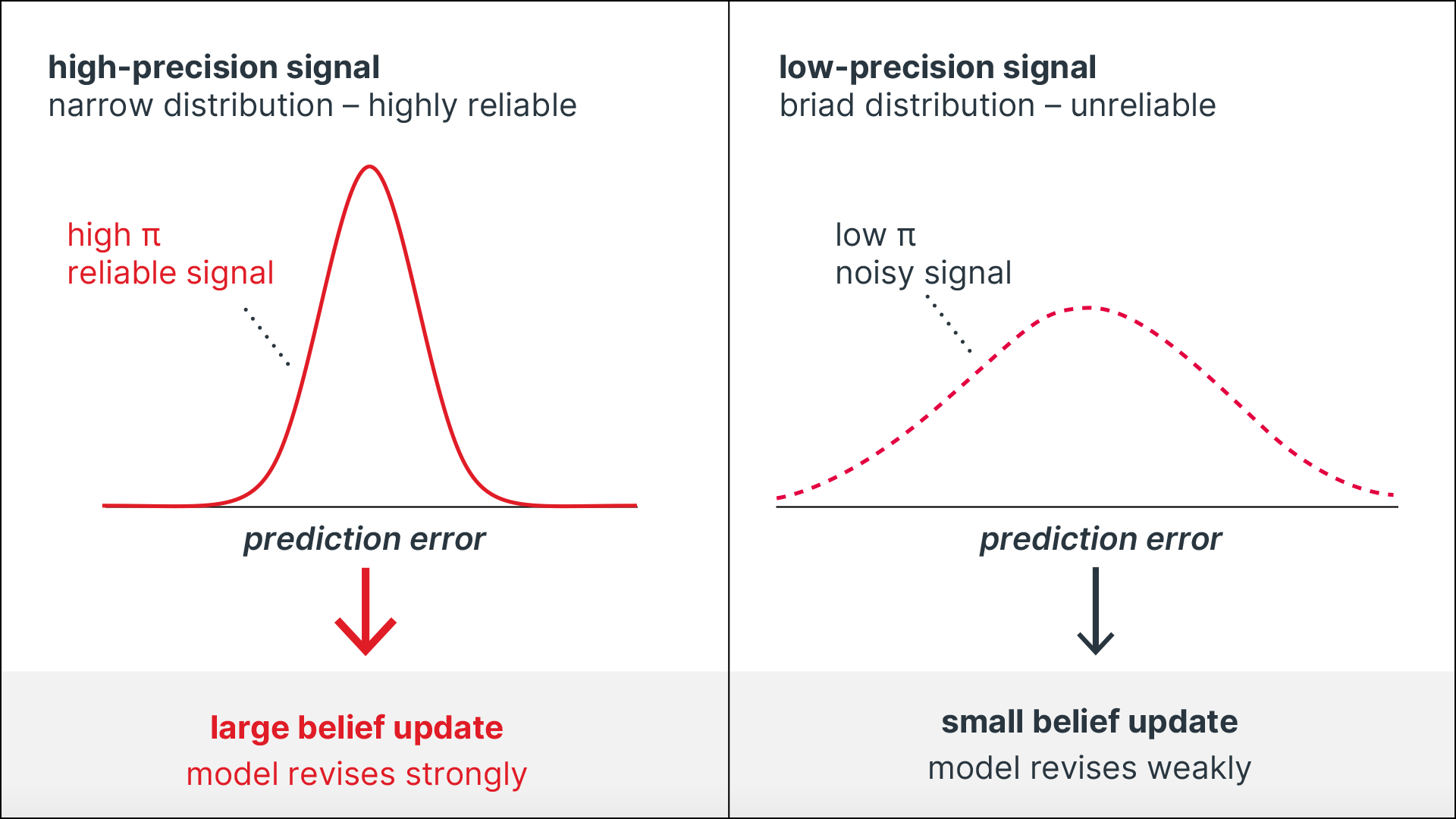
Precision weighting (Friston, 2005)
Each level maintains a generative model. Not all prediction errors are weighted equally – the brain estimates signal reliability.
Precision = inverse variance of the error signal. Friston links precision weighting to attentional gain: attending to a stimulus raises its precision, amplifying its influence on belief updating.

Friston and colleagues have proposed that this mechanism is, in essence, what attention does. To attend to a stimulus is to increase the estimated precision of its prediction errors, granting them more influence over perception. On this account, attention is not a spotlight that selects information, but a mechanism for calibrating how much different signals are trusted.

Precision weighting also explains why strong expectations can sometimes override incoming evidence entirely. When the brain’s prior is much more precise than the incoming sensory signal, the posterior collapses almost entirely onto the prior. The sensory evidence is discounted: the brain explains away the mismatch rather than updating its model.

A good demonstration is the Hollow Mask Illusion. When we view the concave interior of a rotating face mask, we perceive it as a normal convex face protruding toward us. Our prior expectation that faces are convex is so strong and precise that it dominates over the sensory depth cues indicating concavity. The brain does not update its model. It suppresses the error.

The visualisation below shows how this shift in perceptual inference looks in Bayesian terms. When prior and sensory evidence are similarly reliable, the posterior sits between them. When the prior is highly precise and the sensory signal is weak or ambiguous, the posterior collapses onto the prior – which is what happens when we look at the hollow mask.

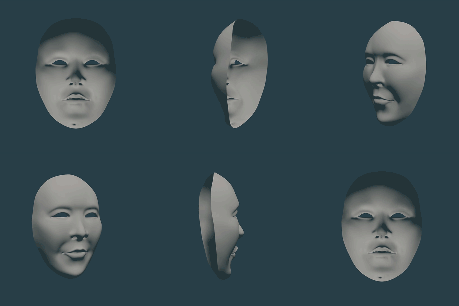
Hollow Mask Illusion

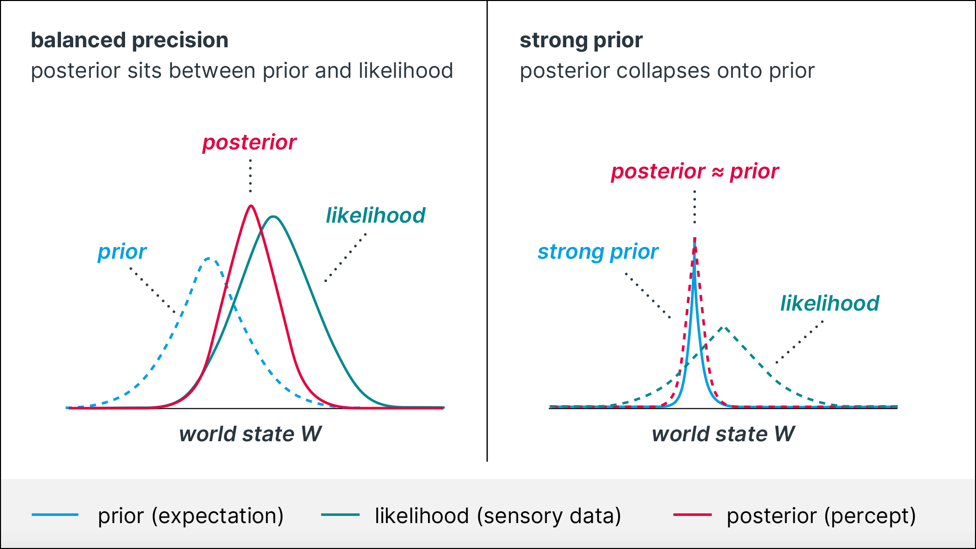
When strong priors override sensory evidence
If the prior is highly precise, the posterior collapses onto it – sensory evidence is discounted.

Authors: Fabian Mueller & William Palmer

References

Yuille, A., & Kersten, D. (2006). Vision as Bayesian inference: analysis by synthesis? Trends in Cognitive Sciences, 10(7), 301-308. https://doi.org/10.1016/j.tics.2006.05.002

Helmholtz, H. von (1867). Handbuch der physiologischen Optik [Handbook of Physiological Optics], Volume 3. Leipzig: Leopold Voss.

Rao, R. P. N., & Ballard, D. H. (1999). Predictive coding in the visual cortex: A functional interpretation of some extra-classical receptive-field effects. Nature Neuroscience, 2(1), 79-87. https://doi.org/10.1038/4580

Friston, K. (2005). A theory of cortical responses. Philosophical Transactions of the Royal Society B: Biological Sciences, 360(1456), 815-836. https://doi.org/10.1098/rstb.2005.1622

Yildirim, I., Belledonne, M., Freiwald, W., & Tenenbaum, J. (2020). Efficient inverse graphics in biological face processing. Science Advances, 6(10), eaax5979. https://doi.org/10.1126/sciadv.aax5979

Griffiths, T. L., Chater, N., Kemp, C., Perfors, A., & Tenenbaum, J. B. (2010). Probabilistic models of cognition: Exploring representations and inductive biases. Trends in Cognitive Sciences, 14(8), 357–364. https://doi.org/10.1016/j.tics.2010.05.004